Spatial Prisoner’s Dilemma for the Course Evolutionary Biology 2025/2026

Idea

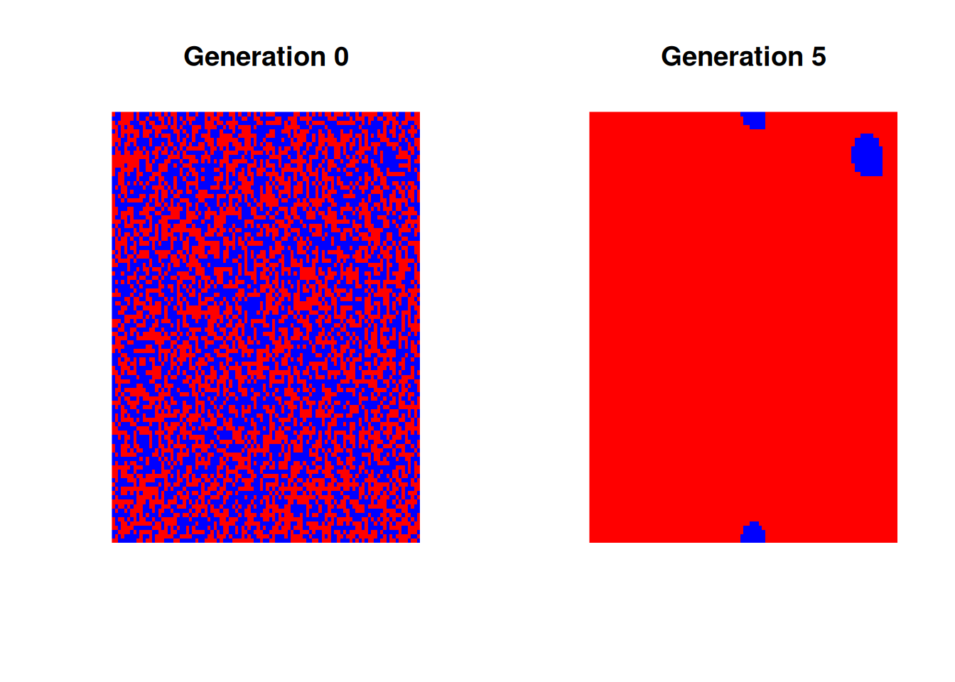
In the section of Evolutionary Game Theory of the Evolutionary Biology course we explore during the course several mechanisms promoting cooperation, following Nowak’s 2006 five rules. The spatial Prisoner’s Dilemma probably captures better than any other mechanism the essence of positive assortment/viscosity in a very visual way: in these simple simulations on a toroidal lattice cooperators survive sticking in “blue bubbles” where they cooperate among each other and are seldom (only at the border) exploited by the defectors.

Simulation

# Spatial Prisoner's Dilemma on a toroidal lattice

set.seed(1)

N <- 100
generations <- 5
T <- 1.5
R <- 1
P <- 0
S <- 0

# 1 = cooperator, 0 = defector
grid <- matrix(sample(c(0,1), N*N, replace=TRUE), N, N)

wrap <- function(i, N){
  if(i < 1) return(N)
  if(i > N) return(1)
  return(i)
}

pd_payoff <- function(a, b){
  if(a==1 && b==1) return(R)
  if(a==1 && b==0) return(S)
  if(a==0 && b==1) return(T)
  if(a==0 && b==0) return(P)
}

compute_fitness <- function(grid){

  N <- nrow(grid)
  fitness <- matrix(0, N, N)

  for(i in 1:N){
    for(j in 1:N){

      payoff <- 0
      count <- 0

      for(di in -1:1){
        for(dj in -1:1){

          if(di==0 && dj==0) next

          ni <- wrap(i+di, N)
          nj <- wrap(j+dj, N)

          payoff <- payoff + pd_payoff(grid[i,j], grid[ni,nj])
          count <- count + 1
        }
      }

      fitness[i,j] <- payoff / count
    }
  }

  fitness
}

update_grid <- function(grid, fitness){

  N <- nrow(grid)
  new_grid <- grid

  for(i in 1:N){
    for(j in 1:N){

      best_fit <- fitness[i,j]
      best_strategy <- grid[i,j]

      for(di in -1:1){
        for(dj in -1:1){

          ni <- wrap(i+di, N)
          nj <- wrap(j+dj, N)

          if(fitness[ni,nj] > best_fit){
            best_fit <- fitness[ni,nj]
            best_strategy <- grid[ni,nj]
          }
        }
      }

      new_grid[i,j] <- best_strategy
    }
  }

  new_grid
}

plot_grid <- function(grid, title=""){

  image(
    t(apply(grid,2,rev)),
    col=c("red","blue"),
    axes=FALSE,
    main=title
  )
}

# Plot initial configuration
par(mfrow=c(1,2))

plot_grid(grid, "Generation 0")

# Run simulation
for(g in 1:generations){
  fitness <- compute_fitness(grid)
  grid <- update_grid(grid, fitness)
}

# Plot final configuration
plot_grid(grid, paste("Generation", generations))